¶ AI Optimizer — Settings Reference
On the portal's AI Optimizer page, you can configure the optimizer with information about your system.
Each parameter below is described at two levels:
- Full description — what it means and why it exists
- Settings hint — the short tooltip to better understand the effect of the setting
Parameters that are physical hardware specifications (inverter size, battery capacity, panel mounting) are described but have no Effect of changing section — they must reflect reality and cannot be freely tuned. Parameters that control optimizer behaviour include an Effect of changing section.
¶ General
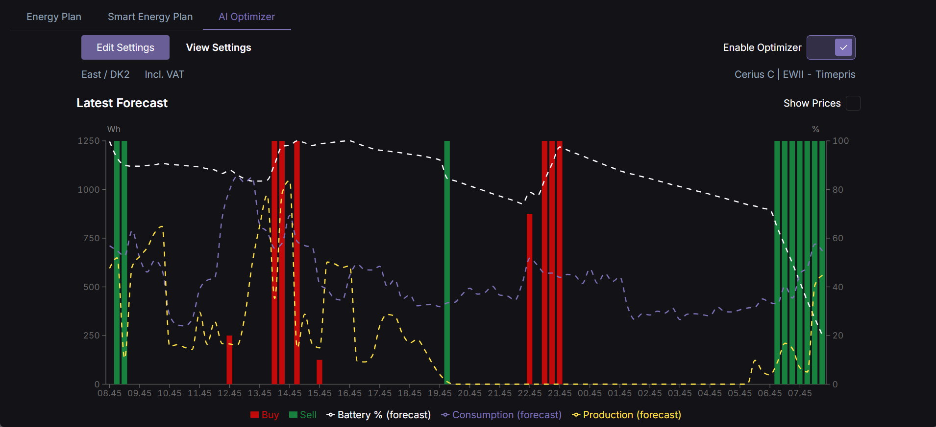
Enable optimization
Activate/deactivate AI optimization as you prefer. Your energy plan will still run, but it will no longer be updated automatically.
Required: To enable the AI optimizer, the energy plan needs to be activated, since the AI optimizer simply updates this plan to fit the current scenario. If the energy plan is not activated, plans will still be generated, but not executed.
¶ Inverter
The inverter converts electricity between the battery/solar (DC) and the grid (AC). These values must match the nameplate data of your physical device.
¶ Rated power
Unit: Watt
Maximum amount of power your inverter can push to the grid or pull from the grid at any moment — the "speed limit" of your inverter. A 12,000 W (12 kW) inverter can export up to 12 kW continuously.
Settings hint: Maximum AC output power of your inverter in watts. Found on the inverter nameplate or datasheet.
¶ Max charge power
Unit: Watt
Maximum rate at which the inverter can draw power from the grid when charging. Typically the same as rated power. Leave blank unless a known lower limit applies.
Settings hint: Maximum grid draw when charging, in watts. Leave blank unless a known lower limit applies.
¶ Max discharge power
Unit: Watt
Maximum rate at which the inverter can export to the grid or supply your home when discharging. Typically the same as rated power. Leave blank unless a known lower limit applies.
Settings hint: Maximum export/supply rate when discharging, in watts. Leave blank unless a known lower limit applies.
¶ Trading
Controls what the optimizer is allowed to do with the grid, which tariff it uses for pricing, and any limits set by your electricity agreement.
¶ Enable buy
Gives the optimizer permission to schedule slots where it buys cheap grid electricity to store in the battery. When off, the battery can still charge from solar — just not deliberately from the grid.
Settings hint: Allow the optimizer to buy electricity from the grid to charge the battery.
Effect of changing:
- Off: The optimizer never deliberately charges from the grid; the battery only charges from excess solar. Reduces flexibility on low-sun, high-evening-price days. Financial returns typically decrease.
- On: The optimizer can buy at low-price hours (e.g. night) and sell or self-consume at high-price hours — usually the most profitable mode where prices vary significantly.
¶ Enable sell
Gives the optimizer permission to schedule slots where it discharges the battery to the grid for revenue. When off, the battery still covers self-consumption but won't deliberately export.
Settings hint: Allow the optimizer to sell electricity from the battery back to the grid.
Effect of changing:
- Off: Battery is used only to cover your own consumption; no export earnings. Useful if your grid agreement disallows export or prices are never worth it.
- On: The optimizer can discharge during high-price hours to earn revenue. Works best with a clear daily price peak.
¶ Buy loss
Unit: DKK/kWh
Extra cost added on top of the grid buy price to account for real-world losses — inverter heat, round-trip inefficiency, wear. E.g. with a 5% cycle loss and a 2 kr/kWh price, a buy_loss of 0.10 makes buying appear to cost 2.10 kr/kWh. Makes the optimizer less aggressive about buying.
Settings hint: Extra cost per kWh (DKK) added to buy price to account for losses. Use 0 if unknown.
Effect of changing:
- Higher: Optimizer requires a bigger buy/sell price gap before committing — fewer buy slots. Useful if real-world returns are lower than predicted.
- Lower (toward 0): Optimizer treats buying as cheaper and schedules more buy actions — risk of over-trading if real losses aren't zero.
¶ Sell loss
Unit: DKK/kWh
Cost subtracted from the sell price to represent discharge-side losses. Works like buy_loss but reduces the apparent value of selling — the optimizer only sells when the net price still makes it worthwhile.
Settings hint: Cost per kWh (DKK) deducted from sell price to account for losses. Use 0 if unknown.
Effect of changing:
- Higher: Optimizer demands higher sell prices before discharging — fewer sell slots. Good where real conversion losses are measurable or self-consumption is preferred.
- Lower (toward 0): Optimizer treats selling as more profitable and discharges more freely.
¶ No-buy windows
Time windows during which the optimizer is completely blocked from grid-buy (charge) actions, regardless of price. Times use the trading.timezone setting (default Europe/Copenhagen); ranges can cross midnight (e.g. "22:00-06:00"). Useful for grid agreements that charge extra for night imports, or to protect the battery overnight.
Settings hint: Time ranges (local time) when buying from the grid is not allowed. Example: ["22:00-06:00"] blocks overnight charging.
Effect of changing:
- Adding a window: Buying is blocked in those hours, even if cheap electricity is available.
- Removing a window: More flexibility to buy at any hour with a good price.
¶ No-sell windows
Same format as no_buy_windows, but blocks grid-sell (discharge) actions. Useful when your grid agreement restricts export at certain times.
Settings hint: Time ranges (local time) when selling to the grid is not allowed. Example: ["22:00-06:00"] blocks overnight discharge.
Effect of changing:
- Adding a window: No export during those hours; battery preserved for self-consumption or later selling.
- Removing a window: More opportunity to hit peak prices at any hour.
¶ Max sell power
Unit: Watt
Maximum rate the optimizer may export to the grid. Applies only to grid export — not to how much the battery can supply the household. E.g. a 10,000 W inverter with this set to 5,000 W can still deliver up to 10,000 W to cover home consumption; only the grid-bound portion is capped. Usually set by your DSO (Distribution System Operator) agreement. Leave blank for no export limit.
Settings hint: Maximum grid export power in watts, as set in your DSO agreement. Leave blank if unrestricted.
Effect of changing:
- Lower: Optimizer can't export at full inverter power — sells less per slot, spreading income out or losing some potential revenue.
- Higher / removed: Optimizer can export at full inverter speed, maximising revenue per peak slot (only if your agreement permits it).
¶ Max buy power
Unit: Watt
Maximum rate the optimizer may import from the grid. Same idea as max_sell_power_w but for charging; some agreements cap import to protect the local grid. Leave blank for no limit.
Settings hint: Maximum grid import power in watts, as set in your DSO agreement. Leave blank if unrestricted.
Effect of changing:
- Lower: Battery charges more slowly during buy slots — may need more slots to reach target SoC, or may not fully charge before prices rise.
- Higher / removed: Faster charging, filling the battery in a shorter cheap-price window.
¶ Timezone
Tells the system which time zone your buy/sell window times are expressed in. Must be a valid IANA time zone name (e.g. Europe/Copenhagen, Europe/London, America/New_York, UTC). If blank, uses the time zone configured on your user account (also defaults to Europe/Copenhagen).
Settings hint: Time zone for your buy/sell restriction windows. Uses IANA format, e.g. "Europe/Copenhagen".
Effect of changing:
- Local time zone (recommended): Window times match your wall clock; DST shifts are handled automatically.
UTC: Windows are fixed to UTC — e.g. in summer (CEST = UTC+2) a"22:00"UTC window starts at midnight local time. Useful only if you deliberately want UTC-pinned blocks.- Blank: Defaults to
Europe/Copenhagen.
¶ Include VAT
Tells the system whether VAT is actually charged to this user. When true, 25% VAT is added on top of fetched electricity prices before decisions are made. Set false for VAT-exempt users (e.g. businesses that reclaim VAT).
Settings hint: Whether VAT applies to this user's electricity costs. True for most Danish households; false for VAT-exempt businesses.
Effect of changing:
- True → False: Optimizer stops adding VAT. Use only when the user genuinely doesn't pay it — setting this incorrectly makes the optimizer underestimate true cost.
- False → True: VAT is added to all prices before optimizing — correct for ordinary household users.
¶ Supplier
The electricity grid supplier for this user (owns the local distribution network, charges transport fees). Used to look up correct tariff components for the user's area.
Settings hint: Your grid supplier.
¶ Product
The specific electricity product/tariff with the supplier (hourly spot, fixed, time-of-use, etc.). Used to fetch the correct buy and sell prices.
Settings hint: Your electricity product/tariff.
¶ Battery
Physical and operational parameters for your battery storage system.
¶ Capacity
Unit: Wh
Total amount of electricity your battery can store. A 40,000 Wh (40 kWh) battery can, in theory, power a 4,000 W load for 10 hours — in practice you never use 100% of capacity (see lowest_soc). Must match your battery's usable capacity spec.
Settings hint: Usable battery capacity in watt-hours (Wh). Found on the battery datasheet.
¶ Max charge power
Unit: Watt
Maximum rate the battery itself can accept charge. Some chemistries (especially LFP) have a built-in charge limit lower than the inverter could otherwise supply. Note: solar already occupies part of the battery's charge budget — e.g. with a 5,000 W limit and solar already pushing 3,000 W, the inverter can only draw an additional 2,000 W from the grid.
Settings hint: Maximum DC charge rate of the battery in watts.
¶ Max discharge power
Unit: Watt
Maximum rate the battery can deliver power. Older/smaller packs sometimes can't discharge as fast as the inverter can export. Note: solar counts toward total inverter output alongside battery discharge — e.g. a 10,000 W inverter with this set to 3,000 W and solar producing 5,000 W can still export up to 8,000 W total.
Settings hint: Maximum DC discharge rate of the battery in watts.
¶ Lowest SoC
Unit: %
Minimum charge level the optimizer will ever allow. Acts as a reserve for blackout protection and protects battery health, since deep repeated discharges accelerate degradation. Common choice: 20%.
Settings hint: Minimum battery charge level (%) to keep in reserve at all times. Typical value: 20.
¶ Max buy SoC
Unit: %
Highest level the optimizer will deliberately charge to when buying from the grid. Kept below 100% to leave headroom for later solar — predictions are never perfect, and if solar turns out stronger than expected, surplus energy needs somewhere to go. Defaults to 90% if not set.
Settings hint: Maximum charge level (%) when buying from the grid. Leave headroom for daytime solar. Default: 90.
Effect of changing:
- Lower (e.g. 80%): Less aggressive grid charging; more room for solar, but less cheap overnight energy stored.
- Higher (e.g. 95%): More cheap grid electricity stored, but may not have room for all of next day's solar.
¶ Min sell SoC
Unit: %
Lowest level the optimizer will discharge to when selling. Prevents selling the battery fully empty and then having to buy back at a possibly high current price. Setting slightly above lowest_soc gives a safety margin. Defaults to lowest_soc if left at 0. Common reason to raise this: an EV that plugs in unexpectedly while the battery is near-empty from peak selling — the optimizer can't predict unscheduled EV sessions, so this reserve buffers against that.
Settings hint: Minimum charge level (%) when selling to the grid. Prevents selling the battery empty and then buying back. Typical value: 25–35.
Effect of changing:
- Lower (closer to
lowest_soc): More energy sold per peak slot, maximising revenue, but less buffer — risk of buying back at a poor price if consumption is higher than predicted. - Higher: Larger reserve retained when selling. Safer, less revenue per sell cycle.
¶ Solar
Configuration for your solar panel installation. Location and panel specs must reflect your physical installation. Only set these if you have solar panels.
¶ Enabled
On/off switch for solar prediction. When false, the optimizer assumes no solar production at all. Only use this for sites genuinely without panels — if panels exist but this is disabled, the optimizer can't predict daytime production and may buy from the grid during hours solar would have covered for free.
Settings hint: Turn off only if there are no solar panels on this site.
Effect of changing:
- False: Plans as if there's no solar — may cause unnecessary grid purchases. Only correct for sites without panels.
- True: Solar production is predicted and used in the plan; avoids buying during daylight hours solar covers, and factors in excess solar for selling decisions.
¶ Location
GPS coordinates of your solar installation (filled automatically if you select on the map). Used to calculate sunrise/sunset, sun angle throughout the day, and to fetch local weather/cloud forecasts. Accuracy matters — a wrong location can shift predicted sunrise or model the wrong sun angle.
Settings hint: GPS coordinates of your solar panels. Used for sun angle and weather forecast.
¶ Force physics
Normally the system learns from your panels' own historical output, adjusted for expected cloud cover — the most accurate method, since it captures shading, degradation, and installation-specific losses. When enabled, it switches to a purely mathematical model (pvlib + MET Norway cloud forecast) that ignores history. Useful for brand-new installations with no history yet, or known-corrupted historical data.
Settings hint: Force the physics-based solar model instead of learning from historical output. Use only if history is unavailable or unreliable.
Effect of changing:
- True: Physics model used. Generally less accurate for established systems (unaware of local shading/degradation) but more reliable for new installations. May over-predict on heavily shaded sites.
- False (default): Predictions learn from actual measured output. More accurate once at least 7 days of history exist.
¶ Rated power
Unit: Watt
Total peak power output of this panel group, as stated on the nameplate — e.g. 20 panels × 300 W = 6,000 W. Used to calculate ideal-condition output, later scaled down by cloud cover and losses.
Settings hint: Total nameplate power of this panel array in watts (e.g. 20 × 300 W panels = 6000 W).
¶ Tilt
Unit: Degrees
Angle of your panels relative to horizontal. 0° = flat, 90° = vertical. Typical Danish roof pitch: 20–40°. Affects how much sunlight hits the panel through the day and year.
Settings hint: Panel angle in degrees. 0 = flat, 90 = vertical. Typical roof pitch: 20–35°.
¶ Azimuth
Unit: Degrees
Direction panels face, meteorological convention: 0° = south, 90° = west, −90° = east, ±180° = north. South-facing gets the most total sunlight in the northern hemisphere; east-facing produces more in the morning, west-facing more in the afternoon.
Settings hint: Direction panels face: 0 = south, 90 = west, −90 = east, ±180 = north.
¶ Performance ratio
A number between 0 and 1 representing real-world conversion efficiency vs. ideal lab conditions. Losses come from inverter conversion, wiring resistance, dirt, temperature, and panel mismatch. New, clean, well-installed systems typically run ~0.80; older or partially shaded systems 0.70–0.75.
Settings hint: System efficiency factor (0–1). 0.80 is a good default. Lower if panels are old, dirty, or shaded.
Effect of changing:
- Lower: Predicts less production per slot — useful if the site consistently under-produces vs. the model (confirmed shading, degradation).
- Higher: Predicts more production — only raise above 0.85 with measured data showing high efficiency, or if the model consistently under-predicts.
¶ Altitude
Unit: Metres
Height above sea level. Higher altitude means thinner atmosphere and slightly higher clear-sky irradiance. Negligible below 200 m (most of Denmark). Set 0 if unknown.
Settings hint: Site elevation above sea level in metres. Use 0 if unknown.
¶ Consumption
Controls how the system predicts household electricity use. Getting this right helps the optimizer avoid over-buying or under-preparing for actual needs.
¶ Aggregation
The system predicts consumption from the last 14 days of measured use, summarised per 15-minute slot. "Median" takes the middle value, ignoring unusual spikes (e.g. an unexpected EV charge); "Mean" averages every reading, so spikes pull the prediction up. Median is default because slight under-prediction is cheaper than over-prediction: under-predicting just means a bit more consumption from battery/grid at spot price, while over-predicting risks buying unnecessary electricity and crowding out solar storage.
Settings hint: How past usage is summarised. "Median" ignores occasional spikes (recommended). "Mean" includes them.
Effect of changing:
- Median (default): Lower, more stable predictions; occasional anomalies don't inflate it. Risk: slight under-prediction.
- Mean: Higher predictions reflecting every unusual event proportionally. Better if consumption is highly variable and spikes genuinely recur.
¶ Weekday weight
Multiplier controlling how much to favour historical days on the same weekday as the day being predicted. 1.0 = all days weighted equally; 3.0 = same-weekday days count three times as much. Useful where consumption differs significantly by weekday (e.g. working from home certain days).
For most users, raising this doesn't help in practice — consumption is driven more by price response and unpredictable appliance/EV use than a stable weekly pattern, and narrowing the historical pool this way can make estimates noisier. Default of 1.0 is correct for most sites.
Settings hint: How much to favour same-day-of-week history. 1.0 = equal weight (recommended for most users). Increase only if your weekday/weekend usage is very consistent and significantly different.
Effect of changing:
- Higher (e.g. 3–5): More day-of-week-specific predictions; can help sites with stable weekly routines, but needs 2–3+ weeks of history and isn't beneficial for most users.
- Lower (1.0): All days treated equally — more stable with limited history. Recommended default.
¶ Temperature correction
Adjusts consumption predictions based on outdoor temperature. The system checks whether your historical consumption correlates with cold weather (suggesting a heat pump or electric heating); if the correlation is strong enough, cold-day predictions scale up and warm-day predictions scale down. Stays inactive if the correlation is weak (R² below 0.2), so it's safe to enable on any site. Requires latitude/longitude to find the nearest weather station.
Settings hint: Adjust consumption predictions based on forecast temperature. Useful if you have a heat pump or electric heating. Requires location coordinates.
Effect of changing:
- Enabled: Cold days → higher predicted consumption and more reserved battery capacity, reducing aggressive selling. Warm days → lower predictions, allowing more selling. Only takes effect if a real temperature-consumption link exists in the data.
- Disabled (default): Predictions use historical patterns only, regardless of forecast. Works well for sites without significant heating loads.
¶ Location
GPS coordinates of your home, used to find the nearest weather station when temperature correction is enabled. Can be the same as your solar coordinates if the installation is at the same address.
Settings hint: Location of your home for fetching local temperature data. Required when temperature correction is on.
¶ Optimizer Settings
Internal tuning parameters controlling how the optimizer solves the daily plan. These affect computation speed and solution quality, not your physical hardware.
¶ Power increment
Unit: %
The optimizer works in discrete steps rather than considering every possible power level — e.g. 0%, 10%, 20%… with a default step of 10. Smaller steps give finer control but take longer to compute.
Settings hint: Step size (%) for power decisions. Smaller = more precise but slower to compute. Default: 10.
Effect of changing:
- Smaller (e.g. 5%): More precise buy/sell tuning, slightly better financial results, but slower — risk of timeout if
time_limitis short. - Larger (e.g. 20%): Faster, but the plan looks blockier — full power or nothing, less granularity.
¶ SoC increment
Unit: %
Same concept as power_increment but applied to battery SoC targets — default step of 10% (20%, 30%, 40%, etc.). Smaller steps give a more accurate SoC trajectory but need more computation.
Settings hint: Step size (%) for battery charge level tracking. Smaller = more accurate but slower. Default: 10.
Effect of changing:
- Smaller (e.g. 5%): More precise SoC tracking — useful for tight constraints (e.g.
lowest_soc= 25,min_sell_soc= 30) where a 10% step misses the target. - Larger (e.g. 20%): Faster, but the SoC trajectory is approximated more coarsely.
¶ MIP relative gap
The optimizer stops searching once its solution is within this percentage of the mathematically perfect answer. 0.01 = stops within 1% of optimal. Lower values (e.g. 0.001) force more searching for a closer-to-perfect solution but take longer; higher values (e.g. 0.05) let it stop sooner with a plan that may be up to 5% below optimal.
Settings hint: How close to perfect the plan must be before the solver stops. 0.01 = within 1% of optimal. Lower = better but slower.
Effect of changing:
- Lower (e.g. 0.001): Searches harder/longer — marginally better results, but may regularly hit
time_limitbefore finishing. - Higher (e.g. 0.05): Stops sooner — faster plans, possibly a few percent below best possible outcome.
¶ Time limit
Unit: Seconds
Maximum time the optimizer may spend solving a plan; returns the best plan found so far if it hits this limit. Runs once per hour, so a 10-second limit leaves plenty of margin. Longer limits mainly help complex scenarios (large batteries, fine increments).
Settings hint: Maximum seconds the solver can run per plan. Best plan found within this time is used. Default: 10.
Effect of changing:
- Longer (e.g. 30s): More time to find a better plan — useful with small increments (5%) or large battery/inverter combinations.
- Shorter (e.g. 5s): Faster, but may return a suboptimal solution more often. Rarely worth going below 10s.
¶ Clip threshold
Inverters and grid agreements sometimes impose a hard export limit — production above it is "clipped" and wasted. The system detects this by treating any historical slot at or above this fraction of the site's all-time peak (default 0.92 = 92%) as clipped and excluding it from predictions, so artificially capped readings don't make the system underestimate true panel output.
Settings hint: Historical solar slots at or above this share of your site's measured peak are assumed clipped (export-limited) and excluded from predictions. Default: 0.92. Only adjust if you see prediction errors around midday.
Effect of changing:
- Lower (e.g. 0.85): Excludes more historical slots as clipped — useful for aggressive clipping, but risks excluding too much good data.
- Higher (e.g. 0.97): Excludes fewer slots — use only if the site never clips, or the default is wrongly excluding good readings.
¶ Input Override
Controls which device node historical data is read from. Useful when a device has been replaced and old data lives under a different node ID.
¶ Enabled
Normally historical data (solar production, consumption, current battery state) is read from the same device as your identity node. When enabled, it's instead read from the node specified by input_override.nodeID — useful after a device replacement, where the old device still holds the needed history. The write side (new device) is set separately under output_override or user.
Settings hint: When enabled, historical data is read from the override node instead of your identity node. Use after a device replacement.
Effect of changing:
- Enabled with a valid source node: Solar/consumption history and current SoC come from the override node; the plan is still written to the node under
output_override. - Disabled (default): Historical data always comes from
user.nodeID— the normal mode when the same device is both source and target.
Screenshots:
Optimizer Enabled